ggnext

Data visualisations, reimagined, using a next-generation Grammar of Graphics — the familiar grammar, extended with native interactivity, animation, exact data export, and a far larger geom catalog.

S7 · SVG · canvas · 59 geoms

Install

# install.packages("remotes")
remotes::install_github("itsmdivakaran/ggnext")

Quick start

library(ggnext)

p <- ggnext(cars, aes(speed, dist)) +
  geom_point(alpha = 0.6) +
  geom_smooth(method = "lm") +
  labs(title = "Stopping distance rises with speed",
       x = "Speed (mph)", y = "Distance (ft)") +
  theme_minimal()

p                                  # static SVG, shown in the viewer
render(p, file = "plot.svg")       # save it
render(p + interact(), file = "plot.html")   # interactive version
plot_data(p)                       # exactly the values drawn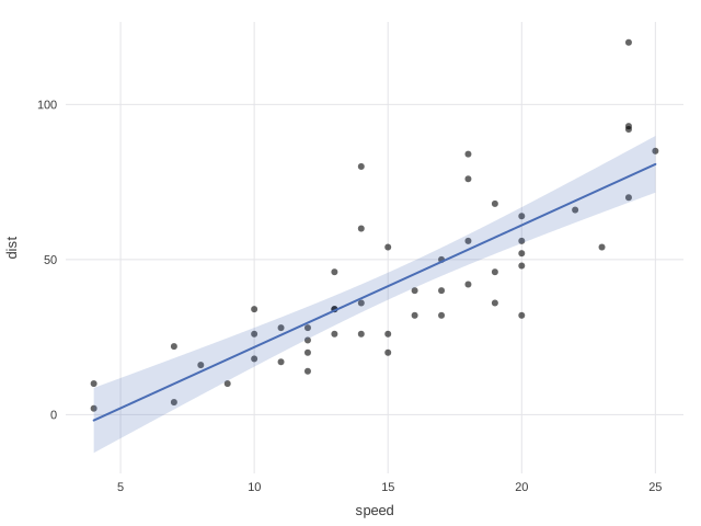

What you get

The grammar you already know

data + aes() + geoms + stats + scales + coords + facets + theme, composed with +. The vocabulary and the muscle memory carry straight over.

One object, two renderers

The same plot renders to a standalone SVG or a self-contained interactive HTML page, from one computed-geometry buffer - so the targets cannot disagree.

Static first, interactive on request

render(p) gives you an image. Adding + interact() opts into tooltips, scroll-zoom, and brush-to-zoom; + animate() adds a frame scrubber.

A much larger catalog

59 geoms in the box: essentials through Sankey, treemap, network, radar, SHAP, ROC, Kaplan-Meier, forest, and CONSORT - no extension hunting.

Exact data export

plot_data(p) returns precisely the values drawn - post-stat, post-position, post-facet - so you can publish the numbers beside the figure.

Pipe-native, if you prefer

Every constructor that takes an argument also accepts a plot as its first pipe stage: p |> geom_point() |> theme_minimal() runs the same as p + geom_point() + theme_minimal().

A linter for the plot itself

validate_plot() checks for common statistical-graphics mistakes - categorical y on a continuous geom, a sqrt scale fed negative values, an unreadable legend - before the figure ships.

Themes and deep customization

Six presets plus 35 theme settings, custom palettes, titles, axis breaks, labels, transforms, and limits.

The grammar

Every plot is data + aes() + layers + scales + coord + facet + theme, composed with +. Plots are immutable values: adding a component returns a new plot, so partial specifications can be shared and forked freely.

ggnext(mpg_like, aes(displ, hwy, color = class)) +
  geom_point(size = 3) +
  facet_wrap(class) +
  scale_y_continuous(name = "Highway MPG", breaks = c(20, 30, 40)) +
  coord_cartesian() +
  interact(tooltip = c("model", "hwy"), brush = TRUE) +
  theme_modern()

See the Guide for a walkthrough, the Gallery for 58 worked examples, or the Cookbook for every function and option demonstrated end to end.

Pipe sugar

+ stays the grammar's one true composition operator - it's what lets a theme_minimal() + theme(legend.position = "bottom") bundle be built once and reused across a report's plots, or a list of layers folded in with Reduce(`+`, layers, p). Neither has a clean pipe equivalent, so + is not going anywhere. But a straight-line pipeline reads better piped, so every constructor that takes an argument also accepts a plot as its first pipe stage - a call-site convenience layered on the same grammar, not a second one.

cars |>
  ggnext(aes(speed, dist)) |>
  geom_point(alpha = 0.6) |>
  geom_smooth(method = "lm") |>
  labs(title = "Stopping distance rises with speed")

is exactly the + chain above, same object. Non-standard evaluation is preserved, so p |> facet_wrap(cyl) resolves cyl against the data exactly as p + facet_wrap(cyl) always has. A handful of constructors that take no arguments at all - theme_minimal(), coord_flip(), and the other bare theme presets - have no slot to route a piped plot through, so those stay +-only.

Plot validation

The grammar will happily build a plot that misleads: a point geom on a categorical y that should have been a boxplot, a sqrt() scale fed negative values, a legend with forty color levels no one can read. validate_plot() checks for exactly this class of mistake; plot_check() does the same but prints the report and returns the plot unchanged, so it drops into a pipeline without breaking it. It's a heuristic, not a guarantee - it flags what commonly goes wrong, not what's definitely wrong with this particular plot.

mtcars |>
  ggnext(aes(mpg, as.character(cyl))) |>
  geom_point() |>
  plot_check()
#> ⚠ GeomPoint-based layer maps y to a categorical column; consider
#>   geom_boxplot(), geom_violin(), or geom_bar() instead.

Interactivity

Interactivity is an additive grammar verb, not a separate package or a post-hoc conversion. + interact() switches the default render target to a self-contained HTML page - vanilla JavaScript, no CDN - driven by the same geometry buffer the SVG writer consumes.

render(p)                                  # static SVG (default)
render(p + interact())                     # tooltips + zoom + brush
render(p + interact(tooltip = c("model"))) # tooltip from data columns
render(p + animate(year))                  # frame scrubber

Credits

ggnext takes its vocabulary from Leland Wilkinson’s The Grammar of Graphics and from Hadley Wickham’s ggplot2, whose API design this package deliberately preserves. The extended catalog follows conventions established by the wider R visualisation community — ggridges, ggalluvial, ggraph, treemapify, ggradar, ggstream, ggupset, circlize, GGally, ggbump, ggiraph, gganimate, survminer, DALEX and others. See the credits page for the full list and the algorithm references.

The implementation is independent: it is written on S7 from first principles, and no code is derived from those packages.